Nonlinear latent variable models
ML-inference in non-linear SEMs is complex. Computational intensive methods based on numerical integration are needed and results are sensitive to distributional assumptions.
In a recent paper: A two-stage estimation procedure for non-linear structural equation models by Klaus Kähler Holst & Esben Budtz-Jørgensen (https://doi.org/10.1093/biostatistics/kxy082), we consider two-stage estimators as a computationally simple alternative to MLE. Here both steps are based on linear models: first we predict the non-linear terms and then these are related to latent outcomes in the second step.
\[ \newcommand{\predphi}{\varphi^*} %%\widehat{\varphi} \newcommand{\influ}{\epsilon} %%\widehat{\varphi} \newcommand{\twostage}{2SSEM\xspace} \]
Introduction: the measurement error problem
Measurement error in covariates is a common source of bias in regression analyses. In a simple linear regression setting, let \(Y\) denote the response variable, \(\xi\) the true exposure, for which we only observe replicated proxy measurements \(X_1, \cdots, X_q\), and \(Z\) an additional confounder:
\begin{align*}
Y &= \mu + \beta\xi + \gamma Z + \delta \\\
\xi &= \alpha + \kappa Z + \zeta \\\
X_{j} &= \nu_{j} + \xi + \epsilon_{j}, \quad j=1,\ldots, q,
\end{align*}
where the measurement error terms \(\delta, \zeta, \epsilon_{j}\) are assumed to be independent of the true exposure \(\xi\). Standard techniques, e.g. linear regression (MLE) on \(X_j\) and \(Z\) fails to provide consistent estimates. To see this observe that
\begin{align*} \widehat{\beta}_{MLE} = \frac{\operatorname{\mathbb{C}ov}(Y,X_{j} \mid Z)}{ \operatorname{\mathbb{V}ar}(X_{j} \mid Z)} = \frac{\beta \operatorname{\mathbb{V}ar}(\xi)} {\operatorname{\mathbb{V}ar}(\xi) + \operatorname{\mathbb{V}ar}(\epsilon_{j})} < \beta \end{align*}
In the following, generalizations of the above problem to general latent variable models including non-linear effects of the exposure variable are considered.
Statistical model
For subjects \(i=1,\ldots,n\), we have latent response variable: \(\eta_i=(\eta_{i1},…,\eta_{ip})^t\) non-linearly related to latent predictor: \(\xi_i=(\xi_{i1},…,\xi_{iq})^t\) after adjustment for covariates \(Z_i=(Z_{i1},…,Z_{ir})\)
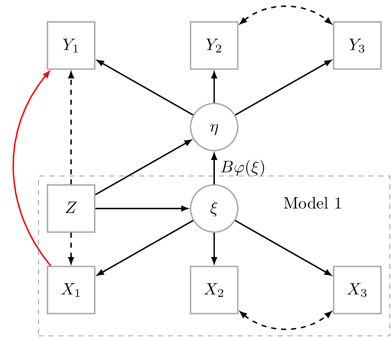
\begin{eqnarray}\label{stmodel}\tag{1} \begin{array}{lcl} \eta_i & = & \alpha + B \varphi(\xi_i) + \Gamma Z_i + \zeta_i, \end{array} \end{eqnarray}
where \(\varphi\colon\mathbb{R}^p\to \mathbb{R}^l\) is a known measurable function such that \(\varphi(\xi_i)=(\varphi_1(\xi_{i}),…,\varphi_l(\xi_{i}))^t\) has finite variance (see Figure 1). The target parameter of interest parametrizing \(B\in\mathbb{R}^{p \times l}\) describes the non-linear relation between \(\xi_i\) and \(\eta_i\). Note, that \(\varphi\) may also depend on some of the covariates thereby allowing the introduction of interaction terms.
The latent predictors (\(\xi_i\)) are related to each other and the covariates in a linear structural equation:
\begin{eqnarray}\label{stmodel1}\tag{2} \begin{array}{lcl} \xi_i & = & \tilde{\alpha} + \tilde{B} \xi_i+\tilde{\Gamma} Z_i + \tilde{\zeta}_i. \end{array} \end{eqnarray}
where diagonal elements in \(\tilde{B}\) are zero.
The observed variables \(X_i=(X_{i1},…,X_{ih})^t\) and \(Y_i=(Y_{i1},…,Y_{im})^t\) are linked to the latent variable in the two measurement models
\begin{align}
\label{memodely}\tag{3}
Y_i = \nu + \Lambda \eta_i + K Z_i+\varepsilon_i \\\
\label{memodelx}\tag{4}
X_i = \tilde{\nu}+\tilde{\Lambda} \xi_i + \tilde{K} Z_i+ \tilde{\varepsilon}_i,
\end{align}
where the error terms \(\varepsilon_i\) and \(\tilde{\varepsilon}_i\) are assumed to be independent with mean zero and covariance matrices of \(\Omega\) and \(\tilde{\Omega}\), respectively. The Øparameters* are collected into \(\theta=(\theta_1^t, \theta_2^t)^t\), where \(\theta_1=(\tilde{\alpha}, \tilde{B}, \tilde{\gamma}, \tilde{\nu}, \tilde{\Lambda}, \tilde{K}, \tilde{\Omega},\tilde{\Psi})\) are the parameters of the linear SEM describing the conditional distribution of \(X_i\) given \(Z_i\). The rest of the parameters are collected into \(\theta_2\).
Two-stage estimator (2SSEM)
- The linear SEM given by equations (\ref{stmodel1}) and is (\ref{memodelx}) is fitted (e.g., MLE) to \((X_i,Z_i), i=1,\ldots,n\) to obtain consistent estimate of \(\theta_1\).
- The parameter \(\theta_2\) is estimated via a linear SEM with measurement model given by equation (\ref{memodely}) and structural model given by equation (\ref{stmodel}), where the latent predictor, \(\varphi(\xi_i)\), is replaced by the Empirical Bayes plug-in estimate \(\predphi_n(\xi_i) = \mathbb{E}_{\widehat{\theta}_1}[\varphi(\xi_i)\mid X_i,Z_i]\).
Prediction of non-linear latent terms
For important classes of non-linear functions (\(\varphi\)) closed form expressions can be derived for \(\predphi(\xi_i) = \mathbb{E}[\varphi(\xi_i) \vert X_i,Z_i]\). Under Gaussian assumptions the conditional distribution of \(\xi_i\) given \(X_i\) and \(Z_i\) is normal with mean and variance
\begin{align*}
m_{x,z} & = \mathbb{E}(\xi_i \vert X_i, Z_i) = \tilde{\alpha}+\tilde{\Gamma} Z_i +
\Sigma_{X\xi}
\Sigma_X^{-1}
(X_i-\mu_X)\\\
v & = \operatorname{\mathbb{V}ar}(\xi_i \vert X_i, Z_i) =
\tilde{\Psi} - \Sigma_{X\xi}
\Sigma_X^{-1} \Sigma_{X\xi}^t,
\end{align*}
where \(\mu_X= \tilde{\nu} +\tilde{\Lambda}(I-\tilde{B})^{-1} \alpha + \tilde{\Lambda} (I-\tilde{B})^{-1} \tilde{\Gamma} Z_i + \tilde{K} Z_i, \Sigma_X= \tilde{\Lambda} (I-\tilde{B})^{-1} \tilde{\Psi}(I-\tilde{B})^{-1t}\tilde{\Lambda}^{t} +\tilde{\Omega}\) and \(\Sigma_{X\xi}= \tilde{\Lambda}(I-\tilde{B})^{-1} \tilde{\Psi}(I-\tilde{B})^{-1t}\). Note, that the conditional variance does not depend on \(X\), \(Z\).
Polynomials
\begin{eqnarray}\label{polynomial} \begin{array}{lcl} \eta_i & = & \alpha + \sum_{m=1}^k \beta_m \xi_{i}^m+ \zeta_i, \end{array} \end{eqnarray}
Here \(\varphi(\xi_i)=\xi_i^m , (m \in \mathbb{N})\) and conditional means are given by
\begin{eqnarray} \label{poly} \begin{array}{lcl} \mathbb{E}(\xi_i^m \vert X_i, Z_i) =\sum_{k=0}^{[m/2]} , m_{x,z}^{m-2k} , v^{k} , \frac{m!}{2^k k! (m-2k)!} \end{array} \end{eqnarray}
Exponentials
For the exponential function \(\varphi(\xi_i) =\exp(\xi_i)\) an expression can be obtained as \(\exp(\xi_i)\) will follow a logarithmic normal distribution where the mean is
\begin{align*} \mathbb{E}[\exp(\xi_i) \vert X_i, Z_i]= \exp(0.5 v + m_{x,y}) \end{align*}
The conditional mean of functions on the form \(\varphi(\xi_i)=\exp(\xi_i)^m\) is straightforward to calculate as this variable again follows a logarithmic normal distribution.
Interactions
Product-interaction model
\begin{align*} \eta_i & = \alpha + \beta_1 \xi_{1i} + \beta_2 \xi_{2i} + \beta_{12} \xi_{1i} \xi_{2i} + \zeta_i, \end{align*}
now \(\mathbb{E}(\xi_{1i} \xi_{2i} \vert X_i, Z_i)=\operatorname{\mathbb{C}ov}(\xi_{1i}, \xi_{2i} \vert X_i,Z_i) +\mathbb{E}(\xi_{1i} \vert X_i,Z_i) \mathbb{E}(\xi_{2i} \vert X_i, Z_i)\), where terms on the right-hand side are directly available from the bivariate normal distribution of \(\xi_{1i}, \xi_{2i}\) given \(X_i,Z_i\). Regression calibration leads to the correct mean expect that the intercept will be biased as this method will not include the covariance term above.
Splines
A natural cubic spline with \(k\) knots \(t_1<t_2<\ldots <t_k\) is given by
\begin{align*} \eta_i &= \alpha + \beta_0 \xi_{i} + \sum_{j=1}^{k-2} \beta_j f_j(\xi_{i})+ \zeta_i, \end{align*}
with \(f_j(\xi_{i})=g_j(\xi_{i}) - \frac{t_k - t_j}{t_k-t_{k-1}} g_{k-1}(\xi_{i}) + \frac{t_{k-1} - t_j}{t_k-t_{k-1}} g_{k}(\xi_{i}), , j=1,\ldots ,k-2\) and \(g_j(\xi_{i})=(\xi_{i}-t_j)^3 1_{\xi_{i}>t_j}, , j=1,\ldots ,k\). Thus, predictions \(\mathbb{E}[f_j(\xi_{i}) \vert X_i, Z_i]\) are linear functions of \(\mathbb{E}[g_j(\xi_{i}) \vert X_i, Z_i]\), and
\begin{align*}
\mathbb{E}[g_j(\xi_{i})\vert X_i, Z_i]
= &\frac{s}{\sqrt{2 \pi}}[(2s^2+ (m_{x,z}-t_j)^2)
\exp(-[\frac{(m_{x,z}-t_j)}{s\sqrt{2}}]^2)] + \\\
& (m_{x,z}-t_j) [(m_{x,z}-t_j)^2+3 s^2] p_{x,z,j},
\end{align*}
where \(s=\sqrt{v}\) and \(p_{x,z,j}=P(\xi_{i}>t_j \vert X_i, Z_i)=1-\Phi( \frac{t_j-m_{x,z}}{s})\).
Relaxing distributional assumptions
Let \(G_i \sim \mbox{multinom}(\pi)\) be class indicator \(G_i\in\{1,\ldots,K\}\), and \({\xi_i}\) the \(q\)-dim. latent predictor from the mixture
\begin{align*} {\xi_i} = \sum_{i=1}^{K}I(G_i=k){\xi}_{ki} \end{align*}
with \(\tilde{\zeta}_{ki} \sim N(0, \tilde{\Psi}_k)\) where \(\xi_{ki} = \tilde{\alpha}_k + \tilde{B} \xi_{ki}+\tilde{\Gamma} Z_i + \tilde{\zeta}_{ki}\). Assuming \(G_i\) to be independent of \((\tilde{\zeta}_{1i},…,\tilde{\zeta}_{Ki})\) and \((\varepsilon_i, \tilde{\varepsilon}_i)\),
\begin{align*}
\begin{array}{lcl}
\mathbb{E}[\varphi(\xi_i)\vert
X_i,Z_i] &=& \mathbb{E} \{ \mathbb{E} [\varphi(\xi_i)\vert X_i,Z_i,G_i] \vert X_i,Z_i \}\\\
&=& \sum_{k=1}^{K} P(G_i=k \vert X_i,Z_i) , \mathbb{E}
[\varphi(\xi_{ki})\vert X_i,Z_i,G_i=k]\\\
&=& \sum_{k=1}^{K} P(G_i=k \vert X_i,Z_i) , \mathbb{E}
[\varphi(\xi_{ki})\vert X_i,Z_i].
\end{array}
\end{align*}
Results can be extended also to the case where \(\pi\) depends on covariates. Under regularity conditions (Redner 1984) the MLE of the stage 1 mixture model is regular and asymptotic linear (RAL).
Asymptotics
Theorem. Under correctly specified model 2SSEM will yield consistent estimation of all parameters \(\theta\) except for the residual covariance, \(\Psi\), of the latent variables in step 2.
Proof: (intuitive version - linear models and Berkson error)
Let \(Y = \alpha + \beta X + \epsilon\) with Berkson error \(X = W + U\) and \(\operatorname{\mathbb{C}ov}(W, U) = 0\). Let \(Y = \alpha + \beta W + \widetilde{\epsilon}\). Berkson error does not lead to bias in \(\beta\), but residual variance is too high Follows from noting that we have Berkson error in the second step: \(\eta_i = \alpha + B\varphi(ξ_i) + \Gamma Z_i + \zeta_i\). Iterated conditional means: \(\operatorname{\mathbb{C}ov}\{\mathbb{E}\varphi(\xi)|X, Z], \mathbb{E}[\varphi(\xi)|X, Z] − \varphi(\xi_i)\} = 0\).
Assume that we have i.i.d. observations \((Y_i, X_i, Z_i), i=1,\ldots,n\), and we also restrict attention only to the consistent parameter estimates i.e., \(\theta_2\) does not contain any of the parameters belonging to \(\Psi\).
We will assume that the stage 1 model estimator is obtained as the solution to the following score equation:
\begin{align*}\label{eq:U1} \mathcal{U}_1(\theta_1; X, Z) = \sum_{i=1}^n U_{1}(\theta_1; X_i, Z_i) = 0, \end{align*}
and that
- The estimator of the stage 1 model is consistent, linear, regular, and asymptotic normal.
- \(\mathcal{U}\) is twice continuous differentiable in a neighbourhood around the true (limiting) parameters \((\theta_{01}^T,\theta_{02}^T)^T\). Further, \[ n^{-1}\sum_{i=1}^n \nabla U_2(Y_i,X_i,Z_i; \theta_1, \theta_2) \] converges uniformly to \(\mathbb{E}[ \nabla U_2(Y_i,X_i,Z_i; \theta_1, \theta_2)]\) in a neighbourhood around \((\theta_{01}^T,\theta_{02}^T)^T\),
- and when evaluated here \(-\mathbb{E}(\nabla U_2)\) is positive definite.
This implies the following i.i.d. decomposition of the two-stage estimator
\begin{align*}
\sqrt{n}(\widehat{\theta}_2(\widehat{\theta}_1) - \theta_2)
&= n^{-\tfrac{1}{2}}
\sum_{i=1}^n \xi_2(Y_i,X_i,Z_i; \theta_2) \\\
& + n^{-\tfrac{1}{2}}
\mathbb{E}[-\nabla_{\theta_2} U_2(Y,Z,X; \theta_2,\theta_1)]^{-1} \\\
&\times \mathbb{E}[\nabla_{\theta_1}U(Y,Z,X; \theta_2,\theta_1)]
\sum_{i=1}^n\xi_{1}(X_i,Z_i; \theta_1) + o_p(1) \\\
&=
n^{-\tfrac{1}{2}}\sum_{i=1}^n \xi_3(Y_i,X_i,Z_i; \theta_2,\theta_1) + o_p(1).
\end{align*}
where \(\xi_{1}\) and \(\xi_{2}\) are the influence functions from the stage 1 and stage 2 models.
Implementation
Installation in R:
  library(lava)
  library(magrittr)
Simulation
      f <- function(x) cos(1.25*x) + x - 0.25*x^2
      m <- lvm(x1+x2+x3 ~ eta1,
	       y1+y2+y3 ~ eta2,
	       eta1+eta2 ~ z,
	       latent=~eta1+eta2)
      functional(m, eta2~eta1) <- f

      # Default: all parameter values are 1. Here we change the covariate effect on eta1
      d <- sim(m, n=200, seed=1, p=c('eta1~z'=-1))
head(d)
          x1         x2         x3       eta1         y1         y2         y3
1 -1.3117148 -0.2758592  0.3891800 -0.6852610  0.6565382  2.8784121  0.1864112
2  1.6733480  3.1785780  3.3853595  1.4897047 -0.9867733  1.9512415  2.7624733
3  0.5661292  2.9883463  0.7987605  1.4017578  0.5694039 -1.2966555 -2.2827075
4  1.7946719 -0.1315167 -0.1914767  0.1993911  0.7221921  0.9447854 -1.3720646
5  0.3702222 -2.2445211 -0.3755076  0.0407144 -0.3144152  0.3546089  0.9828617
6 -2.8786355  0.4394945 -2.4338245 -2.0581671 -4.1310534 -5.6157543 -3.0456611
        eta2           z
1  1.7434470  0.34419403
2  0.8393097  0.01271984
3 -0.4258779 -0.87345013
4  0.7340538  0.34280028
5  0.2852132 -0.17738775
6 -3.9531055  0.92143325
Specification of stage 1
m1 <- lvm(x1+x2+x3 ~ eta1, eta1 ~ z, latent = ~ eta1)
Specification of stage 2:
      m2 <- lvm() %>%
	  regression(y1+y2+y3 ~ eta2) %>%
	  regression(eta2 ~ z) %>%
	  latent(~ eta2) %>%
	  nonlinear(type="quadratic", eta2 ~ eta1)
Estimation:
(mm <- twostage(m1, m2, data=d))
                    Estimate Std. Error  Z-value   P-value
Measurements:
   y2~eta2           0.98628    0.04612 21.38536    <1e-12
   y3~eta2           0.97614    0.05203 18.76166    <1e-12
Regressions:
   eta2~z            1.08890    0.17735  6.13990 8.257e-10
   eta2~eta1_1       1.13932    0.15548  7.32770    <1e-12
   eta2~eta1_2      -0.38404    0.05770 -6.65582 2.817e-11
Intercepts:
   y2               -0.09581    0.11350 -0.84413    0.3986
   y3                0.01440    0.10849  0.13273    0.8944
   eta2              0.50414    0.17550  2.87264  0.004071
Residual Variances:
   y1                1.27777    0.18980  6.73206
   y2                1.02924    0.13986  7.35895
   y3                0.82589    0.14089  5.86181
   eta2              1.94918    0.26911  7.24305
  pf <- function(p) p["eta2"]+p["eta2~eta1_1"]*u + p["eta2~eta1_2"]*u^2
  plot(mm,f=pf,data=data.frame(u=seq(-2,2,length.out=100)),lwd=2)
