ODEs with the targeted package using external pointers

Klaus Kähler Holst

Feb 26, 2021 5 min read

Mathematical and statistical software often relies on sequential computations. Examples are likelihood evaluations where it typically is necessary to loop over the rows of the data, or solving ordinary differential equations where numerical approximations are based on looping over the evolving time. When using high-level languages such as R or python such calculations can be very slow unless the algorithms can be vectorized. Fortunately, it is straight-forward to make the implementations in C/C++ and subsequently make an interface to R and python ( Rcpp and pybind11).

<!–more–>

For generic implementations it may be necessary to allow for user-defined functions defined in the high-level language. In R this is straightforward and nicely implemented with the Rcpp::Function type:

// [[Rcpp::export]]
arma::vec f1(arma::vec x, Rcpp::Function f) {
    for (unsigned i=0; i < x.n_elem; i++) {
        x(i) = f(x(i));
    }
    return x;
}

In R we may then call the function as

f1(1:2, log)

          [,1]
[1,] 0.0000000
[2,] 0.6931472

When the R function only needs to be called a few times this may be a reasonable solution. Unfortunately, in long loops this becomes a bottleneck (in fact, it can be much less efficient than the pure R loop) and destroys the whole purpose of moving the code to C++. Instead, the generic C++ code may be based on receiving an external pointer:

using fun_t = std::function<double(double)>;
using funptr_t = Rcpp::XPtr<fun_t>;

// [[Rcpp::export]]
arma::vec f2(const arma::vec &x, funptr_t f) {
    arma::vec res(x.n_elem);
    for (unsigned i=0; i < x.n_elem; i++) {
        res(i) = (*f)(x(i));
    }
    return res;
}

We can then use a user-defined C++ function for example defined as inline code using the function Rcpp::sourceCpp

Rcpp::sourceCpp(code='
#include <Rcpp.h>
using fun_t = std::function<double(double)>;
using funptr_t = Rcpp::XPtr<fun_t>;

double mylog(double x) {
  return std::log(x);
}

// [[Rcpp::export]]
funptr_t make_funptr() {
   return funptr_t(new fun_t(mylog));
}
')

In R we can then call the original C++-function (wrapped as f2) with the external pointer defined with the new exported function make_funptr:

f2(c(1,2), make_funptr())

          [,1]
[1,] 0.0000000
[2,] 0.6931472

The RcppXptrUtils simplifies this even further allowing inline definitions like

ptr <- RcppXPtrUtils::cppXPtr('double foo(double x) { return std::log(x); }')

To benchmark the solutions we can also look at a pure C++ implementation:

// [[Rcpp::export]]
arma::vec f0(const arma::vec &x) {
    arma::vec res(x.n_elem);
    for (unsigned i=0; i < x.n_elem; i++) {
        res(i) = std::log(x(i));
    }
    return res;
}

res <- microbenchmark::microbenchmark(f0(runif(1e4)),
                                      f1(runif(1e4), log),
                                      f2(runif(1e4), make_funptr()))
res

Unit: microseconds
                            expr        min          lq        mean      median
                f0(runif(10000))    305.291    314.2550    334.9816    322.9965
           f1(runif(10000), log) 110729.709 113773.4825 117273.0796 115268.5975
 f2(runif(10000), make_funptr())    580.814    598.5765    625.8117    609.6140
          uq        max neval cld
    353.6605    505.708   100  a
 117718.3525 230688.562   100   b
    626.7095    816.555   100  a

From the benchmark we see a massive improvement with the external pointer method, f2. There is still some overhead compared to the direct C++ implementation, f0, however in most practical situations this will be of a negligible order (in this example the vectorized R version, log(runif(1e4)), is in fact even faster avoiding the overhead of copying results from memory between R and C++).

ODE example

As an example consider the Lorenz Equations \[\frac{dx_{t}}{dt} = \sigma(y_{t}-x_{t})\] \[\frac{dy_{t}}{dt} = x_{t}(\rho-z_{t})-y_{t}\] \[\frac{dz_{t}}{dt} = x_{t}y_{t}-\beta z_{t}\]

There are various excellent (O)DE solvers (R: deSolve, Julia: DifferentialEquations.jl). Here I will illustrate the above techniques using the targeted R-package based on the target C++ library.

The ODE is specified using the specify_ode function

args(targeted::specify_ode)

function (code, fname = NULL, pname = c("dy", "x", "y", "p"))

The differential equations are here specified as a string containing the C++ code defining the differential equation via the code argument. The variable names are defined through the pname argument which defaults to

dy: Vector with derivatives, i.e. the rhs of the ODE, \(y’(t)\) (the result).
x: Vector, with the first element being the time, and the following elements additional exogenous input variables, \(x(t) = \{t,x_{1}(t),\ldots,x_{k}(t)\}\)
y: Dependent variable, \(y(t) = \{y_{1}(t),\ldots,y_{l}(t)\}\)
p: Parameter vector \[y’(t) = f_{p}(x(t), y(t))\]

All variables are treated as armadillo vectors/matrices, arma::mat.

As an example, we can specify the simple differential equation \[y’(t) = y(t)-1\]

dy <- targeted::specify_ode("dy = y - 1;")

This compiles the function and stores the pointer in the variable dy.

To solve the ODE we must then use the function solve_ode

args(targeted::solve_ode)

function (ode_ptr, input, init, par = 0)

The first argument is the external pointer, the second argument input is the input matrix (\(x(t)\) above), and the init argument is the vector of initial boundary conditions \(y(0)\). The argument par is the vector of parameters defining the ODE (\(p\)).

In this example the input variable does not depend on any exogenous variables so we only need to supply the time points, and the defined ODE does not depend on any parameters. To approximate the solution with initial condition \(y(0)=0\), we therefore run the following code

t <- seq(0, 10, length.out=1e4)
y <- targeted::solve_ode(dy, t, init=0)
plot(t, y, type='l', lwd=3)

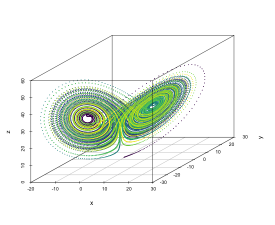
Turning back to the Lorenz Equations we may define them as

library(targeted)
ode <- 'dy(0) = p(0)*(y(1)-y(0));
        dy(1) = y(0)*(p(1)-y(2));
        dy(2) = y(0)*y(1)-p(2)*y(2);'
f <- specify_ode(ode)

With the choice of parameters given by \(\sigma=10, \rho=28, \beta=8/3\) and initial conditions \((x_0,y_0,z_0)=(1,1,1)\), we can calculate the solution

tt <- seq(0, 100, length.out=2e4)
y <- solve_ode(f, input=tt, init=c(1, 1, 1), par=c(10, 28, 8/3))
head(y)

         [,1]     [,2]      [,3]
[1,] 1.000000 1.000000 1.0000000
[2,] 1.003322 1.135177 0.9920639
[3,] 1.013094 1.271279 0.9849468
[4,] 1.029068 1.409156 0.9786954
[5,] 1.051048 1.549630 0.9733721
[6,] 1.078888 1.693496 0.9690541

colnames(y) <- c("x","y","z")
scatterplot3d::scatterplot3d(y, cex.symbols=0.1, type='b',
                             color=viridisLite::viridis(nrow(y)))

To illustrate the use of exogenous inputs, consider the following simulated data

n <- 1e4
tt <- seq(0, 10, length.out=n)  # Time
xx <- rep(0, n); xx[(n/3):(2*n/3)] <- 1  # Exogenous input, x(t)
input <- cbind(tt, xx)

and the following ODE

\[y’(t) = \beta_{0} + \beta_{1}y(t) + \beta_{2}y(t)x(t) + \beta_{3}x(t)\cdot t\]

mod <- 'double t = x(0);
        dy = p(0) + p(1)*y + p(2)*x(1)*y + p(3)*x(1)*t;'
dy <- specify_ode(mod)

With \(y(0)=100\) and \(\beta_0=0, \beta_{1}=0.4, \beta_{2}=-0.5, \beta_{3}=-5\) we obtain the following solution

yy <- solve_ode(dy, input=input, init=100, c(0, .4, -.5, -5))
plot(tt, yy, type='l', lwd=3, xlab='time', ylab='y')